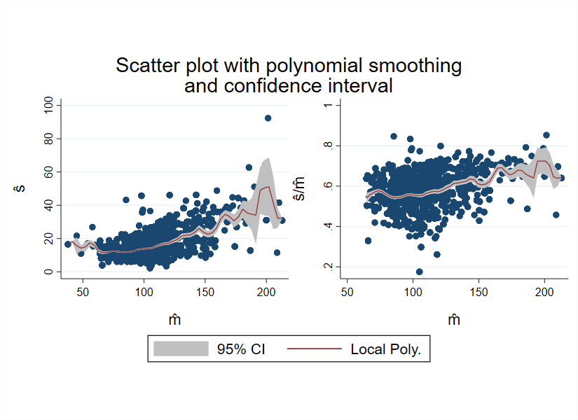
生成上图的Stata代码如下:
* Figure: Scatter plot with polynomial smoothing and confidence interval

**************************************
***                Notes               ***
**************************************
/*
*requires user written command grc1leg
1. findit grc1leg
2. select: grc1leg from http://www.stata.com/users/vwiggins
3. click install
*/

*** Load Data
    use "https://github.com/worldbank/stata-visual-library/raw/master/Library/data/scatter-poly-ci.dta", clear


*** Create First Graph
    sum cons_pae_m_sine, det

    twoway  (scatter cons_pae_sd_sine cons_pae_m_sine if cons_pae_m_sine < `r(p99)') ///
            (lpolyci cons_pae_sd_sine cons_pae_m_sine if cons_pae_m_sine < `r(p99)') ///
         , ///
            legend(off) ///
            xtitle(" " "`=ustrunescape("\u006D\u0302")'", size(large)) ///     m-hat
            ytitle("`=ustrunescape("\u0073\u0302")'" " ", size(large)) ///     s-hat
            xlabel(50 "50" 100 "100" 150 "150" 200 "200") ///
            graphregion(color(white)) bgcolor(white) ///
            name(s_by_mhat)


***C reate Second Graph
    sum cons_pae_m_sine, det

    twoway  (scatter cv cons_pae_m_sine if cons_pae_m_sine<`r(p99)' & cons_pae_m_sine>`r(p1)') ///
            (lpolyci cv cons_pae_m_sine if cons_pae_m_sine<`r(p99)' & cons_pae_m_sine>`r(p1)') ///
         , ///
            ytitle("`=ustrunescape("\u0073\u0302/\u006D\u0302")'" " ", size(large)) ///  s-hat/m-hat
            xtitle(" " "`=ustrunescape("\u006D\u0302")'", size(large)) ///    m-hat
            legend(order(2 3) label(3 "Local Poly.") label(2 "95% CI")) ///
            graphregion(color(white)) bgcolor(white) ///
            name(cv_by_mhat)

*** Combine graphs
    grc1leg s_by_mhat cv_by_mhat ///
            , ///
            row(1) legendfrom(cv_by_mhat) ///
            imargin(0 0 0 0) graphregion(margin(t=0 b=0)) ///
            position(6) fysize(75) fxsize(150) ///
            graphregion(color(white)) plotregion(color(white))

* Have a lovely day!
* Source: https://worldbank.github.io/stata-visual-library/scatter-poly-ci.html